Upscaling with MQTT Workloads Through Data Partitioning

Single Server and the Limits to Growth

Computer software requires hardware resources to operate. These resources come in various forms and quantities serving only three purposes: processing, storage, and transmission.

Processing is quantified by the amount of operations hardware can perform per second. Processing capabilities are provided by a central processing unit (CPU) or various accelerators, such as graphic cards and special-purpose processors, like tensor processing units.

Storage is more diverse. It balances multiple tradeoffs, including size, but also latency of access and reliability. Vast amounts of durable storage where the data survives shutdowns are provided by the disk drives. The main memory of the computer (aka random access memory, or RAM) is frequently a bit smaller, in the range of tens to hundreds of gigabytes, but offers substantially higher speed of accessing the data. Although its content does not survive the shutdown of the computer, low latencies allow software to maintain their runtime data there and maintain high level of responsiveness.

Transmission capabilities of the hardware started to play a role with the introduction of computer networks and gradually acquired significance since more applications started to depend on exchanging the data and collaboratively processing it. Transmission capabilities of a computer system are defined by the medium used to transfer data in the form of analog signals as well as by the protocols that establish the system of slicing and moving the data from one computer to another. 

The synergy of these three fundamental resource types determines how much performance one could expect from the software. Although modern hardware is quite powerful and continues to improve, some applications that serve large user bases (or load in general) often struggle to fit into a single server.

Connected driving platforms of large car manufacturers are a prime example of such an application. Top-tier manufacturers prefer MQTT for its ability to support bidirectional information flow and the highest reliability guarantees. With that choice, their applications have to incorporate an MQTT broker somewhere in the information flow between a car and the processing/storing backends.

We will next do a quick back-of-the-napkin estimation of how much compute and storage resources such a power use-case may demand. Let’s first turn to memory. If every connection requires 30KB RAM then a relatively powerful single AWS r5.4xlarge memory-optimized instance with 32 virtual CPUs and roughly 275 GB can hold approximately 9,17 million connections assuming that the memory is only allocated for connections. Although this may seem like a huge number, this only covers 3% of all the registered vehicles in the USA alone in 2023, and this number will continue to grow. Processing promises to be an even bigger limiting factor if we go for a single server. A reasonable but maybe somewhat optimistic assumption is that every core could process 1,500 messages per second (taking into account that they need to be written to the disk). If that is the case, then r5.4xlarge would be able to cope with 48,000 messages per second which is only 22% of what all the newly registered BMW cars in 2023 in Germany would produce in terms of data if each was sending one message per second. 

Since the scale of the applications relying on MQTT brokers can grow substantially over time, the limits to growth imposed by the single server are something that any broker has to address. Modern brokers achieve this by scaling beyond single server (horizontally) and distributing the load across multiple servers.^[1] 

Venturing Beyond a Single Server: Partitioning to the Rescue

Everyday Partitioning

Scaling horizontally effectively means splitting the work that a single server ought to perform and giving every server in a group a smaller chunk of work. In software engineering, this approach is known as partitioning. Let’s start with a non-software example of partitioning to identify its key characteristics.

Imagine a small family of two working adults living in the same apartment. They have to clean it weekly, do the laundry, get rid of garbage, do small repairs, and so on. Although all these responsibilities might be assigned to only one member of the family, this family member will be overwhelmed after some time. As a result, some duties might end up being forgotten.

Instead of running the risk of failing routines, one could split chores, and, say, agree that one member of the household takes care of cleaning the living room and the kitchen whereas the other one takes care of the bedroom, bathroom, and the hallway. That way the work might get more evenly split between the two family members leaving each with less work to do but still covering all the responsibilities.

There are other dimensions to split the work across, for example, by the kind of activity or based on how much time it takes. Ideally, after partitioning the work, all its pieces can be done by every family member (everyone is equally good at all activities and can substitute one another) and all these splits (partitions) of work are independent of each other.

Building on top of this example, we can discover two key characteristics necessary to perform partitioning, regardless of the domain: a partitioning dimension and a unit identifier. The partitioning dimension in the example could be the category of chore, e.g. cleaning or washing. The identifier needs to be selected in such a way that the activity cannot be misattributed to an incorrect partition. We could select the name that includes the dimension as such an identifier, e.g. vacuum cleaning of the living room, cleaning the kitchen in contrast to washing the sports clothes, washing the car. It is crucial that identifiers of partitioned entities map exactly to one partition resulting from the selected dimension.

Partitioning in MQTT

Let’s return to the MQTT broker and discuss how it handles partitioning.

There are many ways to assign an identifier to the units of work in an MQTT broker. Probably, the most natural one would be to use the client identifier. “Why client identifier?”, you may wonder. A good identifier is something more than simply a unique identifier that we could have tried to extract from messages. A good identifier fulfills expectations for the results of performing work. In case of an MQTT broker, there is a requirement of maintaining the order of messages that are sent from publishers to subscribers via broker.

If the selected partitioning identifiers were as fine-grained as message ids, then two messages (say, m1 and m2) destined for the same client could have landed on two different servers, and then the order of their delivery would be indeterministic. This means that they could have arrived in order m1, m2, but m2, m1 would also be possible. The clients won’t be able to rely on the broker for ordering guarantees then. 

Indeterminism in message ordering forces us to prefer coarser identifiers that have the same granularity as the order of the client messages. Client identifier in that case looks like a good option. Client identifiers have to be unique according to the protocol specification, and the message order is also maintained at the client level. Moreover, if we recall that identifiers need to map to the partitioning dimension in such a way that the partition they end up in is always one and the same, then alphanumeric client identifiers appear to be a good choice as well. 

In the end, we can select alphabet characters as a partitioning dimension and, since the number of characters is finite, we can be sure that every client identifier will be mapped to exactly one partition. We just need to ensure that partitions do not overlap but at the same time cover all the characters of the alphabet. 

For simplicity, imagine client identifiers being generated from the uppercase characters of the alphabet. We will have identifiers like “AAAAB” and something a tiny bit more meaningful like “CLIENT”, or, perhaps, “CONNECTEDVEHICLE”. Then, we split our dimension (alphabet characters) into some partitions. The first partition may become a home for identifiers starting with ‘A’ or ‘B’, the second partition will host identifiers starting with ‘C’ or ‘D’, and so on until we run out of letters. Client with identifier “AAAAB” will then end in the first partition, whereas “CLIENT” and “CONNECTEDVEHICLE” will end up in the second partition.

You probably already see an issue with this approach. If not, think of how balanced such partitions would be. Would the amount of work or data assigned to each partition be roughly the same?

Turns out that such semantic splits might be prone to something known as a hotspot problem. That is, the identifiers are similar forcing the data (or work) to fall into just a handful of all the available partitions. Imagine every MQTT client identifier starting with the sequence “CLIENT”. Then, regardless of what comes after in the identifier, all the clients will be pushed into the same partition. Since partition gets allocated on a single server as per our assumptions, this will negate the effect of partitioning.

Can we do better than that? Certainly. We need to figure out how to allocate units of work (or data) to partitions evenly. There are multiple ways to achieve this, but most of them require a high degree of control over identifiers assignment which one cannot always exercise. Alternatively, one could attempt to rewrite the identifiers on the broker’s side in some way that would increase the distance between them even if they are very similar to each other. This is the path that we take in the next section.

Evening Out the Odds by Hashing the Identifiers

Hash as an Identifier

Our objective for this section is to discover identifiers that do not cluster together on the same server even if they are somewhat similar.

Without modifying the identifiers, that would be a tall order since that would imply severe restrictions on the selection and assignment of identifiers. If the selection and assignment is not centralized, then this approach is doomed. Therefore, to improve the distribution of work or data across the partitions, we need to remap the identifiers; that is, produce a new identifier that is not prone to forming large clusters of data or work on a single server.

Another nuance of identifier remapping is the need to keep the mapping from the original identifier to a new one. If the connections were one-shot (stateless), then there would be no real need to keep the mapping from the original to the new identifier. We could simply assign a new identifier on every reconnect. Since we deal with the stateful connections, we need to provide a way to map the original client identifier to the same new identifier regardless of the mapping attempt. This is a very loose definition of a mathematical function (the same input always produces the same output).

Computer science came up with quite a few functions that remap any kind of identifier into a different one of limited length in such a way that even the high degree of similarity of two original identifiers does not guarantee that they will be similar after remapping. In contrast, these remapping functions may actually drive the identifiers as far apart as possible in the new identifier space.

Such functions are called hash functions, and the process of acquiring the new identifiers is called hashing. The result of applying a hash function to the client identifier (or any kind of identifier) is a hash, a limited-length sequence from some finite set of sequences. The hash does not have any meaning per se but we can endow hash with it. For example, we could say that a hash is a new identifier or, to be more precise, a group of identifiers. 

Due to the sheer size of hash spaces, it is next to impossible to have two different identifiers mapped into the same hash, but this is not completely excluded. For the sake of keeping the discussion easy to follow, we assume the uniqueness of hashes, so every hash can be considered a new identifier. 

Everybody can create their own hash function. A good way to start is to represent the identifier numerically. Although there are not many numerical characteristics of string identifiers, we can still characterize one with its length (e.g. in symbols or glyphs), and then each symbol, in turn, can be characterized by its position in the identifier and in the character table (alphabet or ASCII/Unicode).

For instance, in the word ‘CLIENT’, letter ‘C’ has position 1 and has code 67 in the ASCII table. One could formulate the hash quite arbitrarily as, e.g. sum of letter positions in the word weighted by their positions in the ASCII table, which would mean computing 1 × 67 + 2 × 76 + 3 × 73 + 4 × 69 + 5 × 78 + 6 × 84 and use the resulting 1608 as a hash. Although this number seems to be small, we have to keep in mind that arbitrary-length identifiers could bloat the resulting mapped ID quite quickly.

Since we want to get an even distribution of identifiers across a limited number of servers, we would want to confine the new identifiers (hashes) to some predetermined limited range. We could achieve that with a modulo operation that produces the remainder of division by, for example, the amount of servers. Thus, instead of computing the hash based on only the inputs from the identifier itself, we also constrain the resulting new identifiers not allowing them to be arbitrarily large. If we select the divisor to be 16 then ‘CLIENT’ would end up having hash 08^[2]. ‘CLIENT1’, represented as (1 × 67 + 2  × 76 + 3 × 73 + 4 × 69 + 5 × 78 + 6 × 84 + 7  × 49) mod 16 in remapping, would end up having hash 15.

As we can see, some hash functions can drive even very similar identifiers quite far apart. In the above example, the distance between two modulo results is 7 which is ~44% of the whole hash space. In contrast, the edit distance^[3] between the original identifiers is just one symbol. There are way better hash functions than the ad hoc one introduced before, e.g. the classic MD5 or Murmur. 

Having hashes computed, we are ready to proceed to the next step; that is, mapping these hashes to the partitions. Remember the discussion about the partitioning dimensions? With the introduction of hashes, this part becomes straightforward. It is always the hash of the identifier that serves as a partitioning dimension. The next big question is how to establish the boundaries between the partitions.

Partition Boundaries for Hash Identifiers in Static Deployments

Establishing the boundaries between partitions is not very difficult if we assume that partitions are created on the equally capable servers (in terms of resources, i.e. same AWS instance type). We want the work in each partition to be roughly the same so that the servers have similar levels of resource usage. Thus, having N equally capable servers, we can simply split the continuous space of hashes (it is finite, in our example, it is capped at 16 hashes) into N ranges.

If we divide max hash by N, then we will get the rough count of hashes to allocate to each partition. The resulting value is used as a stride allocating the data to the specific partition. So, the first partition would be responsible for data with hashes between 0 and max/N, the next partition for the data with hashes between max/N + 1 and 2 × (max/N), and so on with the last partition ending at max hash. 

That would have been the end of the story if the number of servers, and, by corollary, partitions, would remain the same forever. That would mean that no server ever fails, no new server is added, and no old server is removed. That, I have to admit, is quite an unrealistic scenario.

What actually happens if the cluster composition changes, say, if we add another node? Let us scrutinize this case with the help of a diagram.

In the figure below, we have the same hash space depicted twice. The above copy spans 3 servers. The below one spans 4. Let’s assume that ‘Server 4’ just got added, so the above hash space division into three partitions (each corresponding to a server) precedes its division into four that is depicted at the bottom of the figure. The hash min and max does not change.

Upon re-partitioning the hash space into 4 partitions, every old server has to send some data even if the receiving server was already part of the cluster from the beginning. These data transfers are required to perform balancing and ensure that the same amount of data stays on every node even if their count increases. As can be seen in the figure (rectangles with red fill), ‘Server 1’ sends roughly one fourth of its data, ‘Server 2’ sends half of its data, and ‘Server 3’ — a daunting ¾ of its data. That’s a lot of communication for adding just one server. In total, we end up reshuffling half the data in the cluster. 

The question that we may want to ask ourselves at this point is: “Can we avoid transferring this huge amount of data on every server addition?” If that was our only option, then there would be no point in hashing in case of cloud deployments — it effectively makes elasticity prohibitively expensive.

To keep the data evenly distributed, theoretically, we would have to move roughly the max / new_server_count portion of the data when the new server is added which is quite a bit less than the original 50% of all the data for the example above. Note that there is no requirement as to where this data needs to come from. Having these two hints in mind, let’s attempt to make the hash-based distribution a bit more scalable in a sense of restricting the amount of data transmitted on cluster composition changes.

Achieving Elasticity With Consistent Hashing

How could we confine the data transfers upon adding or removing nodes? If there only was a way to make the data sticky; that is, to attach it to a specific partition...

To achieve that, we could map both the data (work) identifiers and the unique partition identifiers onto the same hash space. Then, we will have to make a slight twist in assignment of hashed data identifiers to servers. We can do so by agreeing that all the data identifiers hashed into the interval starting with the hash of partition X and ending at the hash of partition Y, belong to partition Y. This partition would then be called responsible for the identifiers falling within the range. That way, the addition of some server Z, whose identifier hashes between Y and X, would result in sending to it only some part of the data which appears between X and Z, and that is stored only on one server — server Y.

By implementing this scheme, we lose control over how many and which exact hashed identifiers each partition hosts. However, with a reasonably well-designed hash function, that should not be a problem since the distribution of both kinds of identifiers (of partitions/servers and of data) will be randomized. 

There is a tiny blind spot in this approach that is worth fixing straight away. Since we represent hash space as linear and since we have no control over where in this space the partition ends up landing, we cannot guarantee that there would be a server in the max hash position. Given our choice to select the closest from the right server (partition) as responsible for hosting the identifiers, which server should we pick in the following case for data point Q? 

We could continue from the beginning and thus assign server X which appears first on the left in the sequence of servers. This effectively means enclosing the hashspace and making it akin to a ring. It is common to represent the hash space as a hash ring. Now, instead of selecting the partition (server) to the right of the hashed identifier of data, we will select one in the clockwise direction (counterclockwise also works). With the following figure, there could be no doubt that server X is responsible for the data item Q.

Given that the hash function remains unchanged, the same identifier, regardless of whether it belongs to the data item or a partition (server), will have exactly the same hash regardless of any conditions. This means that positions of data items and servers (partitions) on the ring remain exactly the same regardless of how many servers and data items are added. 

Once a partition (server) is added or removed, only a fraction of the data on a single server^[4] is transmitted. Only K / N data entities of the total K entities need to be remapped on average with this approach, i.e. the more servers are used in the cluster, the less data will be remapped and transmitted upon cluster composition change. In our example, this 1 / N factor would evaluate to 0.25 as compared to 0.5 that we get when identifiers are mapped to servers based on even distribution in the set of servers ordered by their original ids. Effectively, this halved the traffic on cluster composition change making it both shorter and reducing the possible data transmission costs.

The above ideas underlie the consistent hashing algorithm which was introduced in the late 90s and since then got popularized by its use at the core of Dynamo key-value store at AWS, as well as in the other systems — most prominently, in distributed databases.

There is still a concern of us giving up the control over how many identifiers end up in every partition. “Would not this defeat the purpose of hashing for partitioning in the first place?”. In practice, this would rarely happen if the deployments are large enough. But the problem is that some deployments for smaller use cases are, in fact, quite small compared to the set of all the possible output values of a hash function. Therefore, it is not unheard of to have the partitions (servers) being hashed as depicted below.

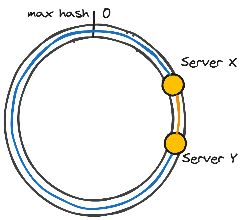Do you see the problem with this distribution of servers on the ring? The range that maps to node X is huge as compared to the range that maps to node Y (blue color used for the range the server X is responsible for, orange — for the range of server Y). Elastic-friendly distribution may in fact become a problem for distributing the work and data if the cluster is small enough. This happens because we gave up control over where the hashed nodes and hashed data identifiers end up being on the hash ring. If only we had more servers…

Mitigating the Shortcomings of Consistent Hashing with Virtual Nodes

Actually, why not? Why not introduce more servers? “But wait a moment, won’t it cost money?”, one may argue. No, since we will introduce virtual servers; that is, every physical server (partition) or a virtual machine is represented by multiple servers (partitions) — for example, 100 or 1000. One could think of this twist as representing each server in terms of units of work that it can perform.

Thus, in our example above if we set the desired number of virtual servers to 5, then, instead of just 2 servers mapped to unique but constant locations on the hash ring, we get 10 such locations. Probability theory allows us to claim that, although still possible, the case when two neighboring nodes on the hash ring are mapped far apart (in comparison to others) got way less probable. As we can see in the example below, the presence of orange ranges (node Y) increased whereas the presence of blue ranges (node X) went down. In total, we have more even distribution of the identifiers across the partitions that belong to these two servers.

But what do we do with the data? We can’t simply send the data to the non-existent virtual servers. However, we can send the data to the corresponding physical server or the virtual machine that this virtual node on the ring was formed from ^[5]. Since we’ve conducted partitioning based on virtual nodes, on average each server (partition) ended up getting roughly the same amount of hash ring that it is responsible for. 

This version of consistent hashing is called consistent hashing with virtual nodes and it is widely used to partition and allocate data in many systems.

With this flavor of consistent hashing, we’ve finally got what we desired:

• scaling beyond single server with partitioning,

• even distribution of work and data across the servers,

• elastic scaling with minimal overhead.

HiveMQ Broker: Consistent Hashing for Better Horizontal Scaling

Being a shared nothing distributed system supporting high availability and scale of up to millions of messages per second, consistent hashing with virtual nodes fares quite high as the most pragmatic choice for HiveMQ Broker. With consistent hashing at the core of data distribution, HiveMQ Broker is able to outgrow a single server and scale horizontally, to the ever-increasing number of servers as the use cases of our customers mature and grow in scale.  

Even though there have been other partitioning schemes developed over time, HiveMQ Broker stands in line with other systems such as Couchbase, Dynamo, Discord, Apache Cassandra, Riak, OpenStack Swift, and many more, including modern vector databases purpose-built for AI workloads, that use consistent hashing to partition their workloads.

References

[1] There are two key reasons to introduce additional instances of the same software. The first one is fault tolerance: when one of the servers fails, there are others to continue serving the load. The second reason is performance: if the load is larger than what a single server can reasonably serve (within some performance constraints like latency), then it needs to be distributed across multiple servers.

[2] Technically, the computation result is 8 but hashes should be the same size so we add 0 at the beginning.

[3] Edit distance between two strings is determined by counting the minimal number of character editing operations (insert, delete, swap) required to transform one string into another.

[4] We skip discussing replication for now, but even then the amount of transmitted data is still bound by the replication factor.

[5] It might be a bit confusing to see the terms ‘virtual machine’ and ‘virtual node’ in the same sentence. Virtual machine is a fraction of hardware resources that a cloud provider offers in the packaging of a server. Virtual node is a more abstract notion relevant only for the data distribution and it simply corresponds to a specific location on the hash ring.